
Summary — Part 1 built a RAG pipeline with chunking, hybrid search and reranking, and Part 2 rebuilt it in Langflow. If retrieval still misses because of internal jargon and document structure, the remaining lever is adapting the retrieval model itself to your data. This post surveys the key ingredient for RAG fine-tuning: synthetic questions plus positive/hard-negative datasets, and lays out a practical build order and its pitfalls. Findings reported in papers are kept separate from my own inferences.
Why build a dataset at all
General-purpose embedding models are strong on public benchmarks, but on internal acronyms, product codes and policy documents they often rank “looks relevant but doesn’t answer” passages too high. If the first-stage candidate set does not contain the answer, no amount of chunking or reranking can recover it.
The problem is that fine-tuning needs (question, correct passage, wrong passage) data, and most organizations have almost none. Hand-labeling thousands of rows is unrealistic, so recent research has converged on synthesizing this data with an LLM.
Components of the training data
| Element | Role | How to get it |
|---|---|---|
| Query | A question a real user might ask | LLM-generated for each document chunk |
| Positive | The chunk that contains the answer | The source chunk the question was written from |
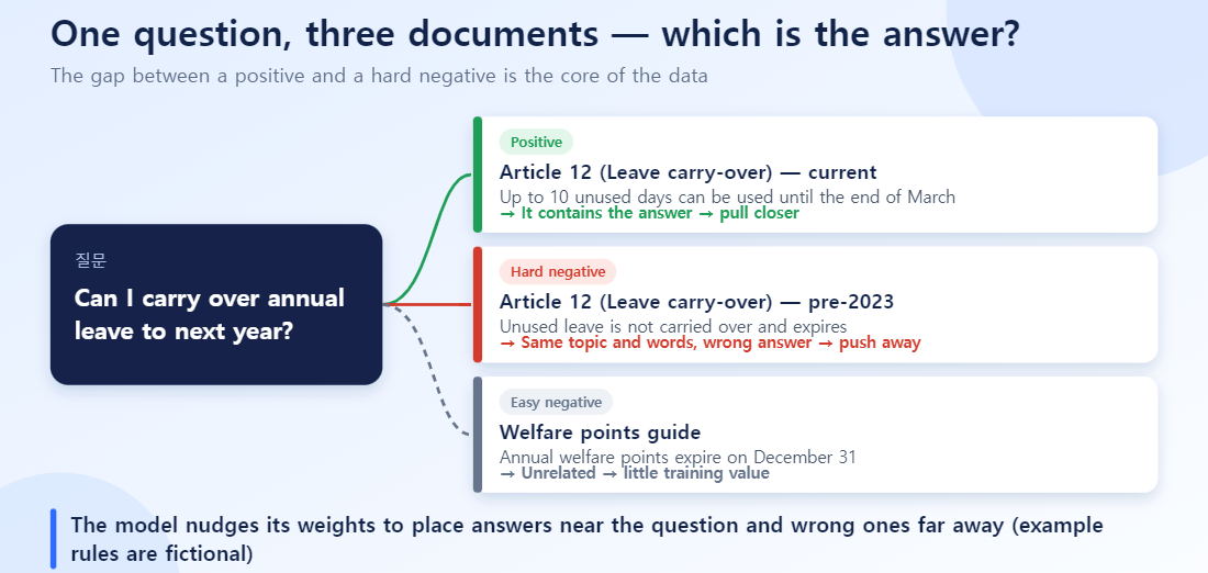
| Hard negative | Similar topic, but no answer | Mined with an existing retriever, or LLM-generated |
| In-batch negative | Other samples in the same batch | Used automatically by the loss function |
Hard negatives are the key. If you only show easy wrong answers (completely unrelated documents), the model just relearns what it already separates. The ability to push away “plausibly wrong” documents comes from hard negatives.
Research survey
1. Synthetic query generation: doc2query → InPars → Promptagator
- InPars uses an LLM to write queries for corpus documents and trains a retriever on the synthetic pairs. The follow-up InPars-v2 filters generated examples with a reranker and swaps the proprietary generator for an open-source one.[1]
- Promptagator replaces a fixed template with a dataset-specific prompt containing a few query-document examples, and reports training small retrieval and reranking models without supervised data.[1]
- InPars+ (2025) fine-tunes the query generator with preference optimization and tunes prompts with DSPy, reporting better retrieval with less reliance on aggressive filtering.[2]
Practical takeaway: Promptagator-style prompting with a handful of domain examples is the cheapest place to start.
2. Quality filtering: consistency filtering
Many generated questions are vague or cannot be answered from the source chunk. A widely used remedy is consistency filtering: run the question through an existing retriever and keep it only if the source chunk lands in the top K.[1] Variants filter by reranker score, as InPars-v2 does.
3. Hard-negative mining and the false-negative problem
Hard negatives are passages that rank high but are not labeled as answers, which is exactly why they are likely to be false negatives: truly relevant passages missing a label.[3]
| Method | Core idea | Cost |
|---|---|---|
| RocketQA (denoised hard negatives) | Use a well-trained cross-encoder to remove likely false negatives from top candidates | Needs a pre-trained cross-encoder |
| NV-Retriever (positive-aware mining) | Use the positive’s relevance score as an anchor and exclude candidates that score too close to it | No extra model needed |
NV-Retriever reports 60.9 on the MTEB retrieval (BEIR) average with this mining, 0.65 points above previous methods.[4] Check the paper itself for the exact threshold formulas.
4. Can an LLM generate the hard negatives directly?
Skipping corpus search and asking an LLM to write hard-negative passages is attractive, but the evidence is mixed.
- Text retrieval (10 BEIR datasets): in a comparison fine-tuning DistilBERT with MNRL, LLM-generated negatives did not consistently beat negatives mined with BM25 or a cross-encoder. Average nDCG@10 was 0.366 for cross-encoder mining, 0.359 for BM25 and 0.314 for the best LLM-only setting (Phi4-14B). Bigger generators were not always better. Limitations: a single student model, one epoch, 10k training passages and no verification of generated negatives.[5]
- Multimodal document reranking: DocReRank goes the other way, generating hard-negative queries per page, and reports that this fixes limits of mining (low diversity, low difficulty, false negatives) and beats existing models.[6]
For text RAG, treating mining as the default and LLM generation as a supplement fits the current evidence. This is my reading of the two studies together, not proof that it generalizes to every domain.
5. Applied to domain RAG
- ALoFTRAG generates and filters synthetic data without labels and fine-tunes with LoRA. It reports average gains of +8.3% citation accuracy and +3.0% answer accuracy across 20 datasets in 26 languages, and positions itself as suitable for sensitive domains because it runs locally without a larger teacher model.[7] Note that the final answer-accuracy gain is much smaller than the retrieval/citation gain.
- On the reranker side, a study that uses only a domain corpus, has an LLM write queries and label positives and hard negatives, then trains a cross-encoder with distillation and contrastive learning, reports large in-domain gains on MedQuAD that generalize out of domain.[8]
Three ways to structure the training data: pairs, triplets, mixed
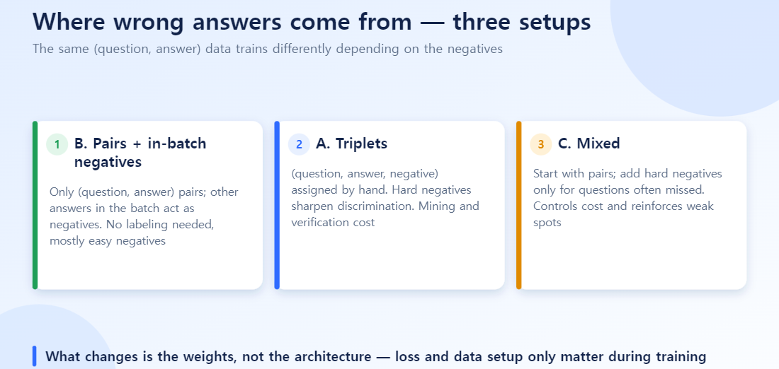
Even with the same (question, answer) data, where the wrong answers come from splits training into three setups. The comparison below assumes MultipleNegativesRankingLoss (MNRL) and InfoNCE-style losses.
| Setup | Data shape | Source of negatives | Strength | Watch out for |
|---|---|---|---|---|
| A. Triplets | (query, positive, negative) | Hand-assigned hard negative plus other samples in the batch | Explicitly pushes away plausibly wrong passages | Mining and verification cost, false negatives |
| B. Pairs + in-batch negatives | (query, positive) | The positives of all other queries in the same batch | No labeling or mining, simple to implement | Mostly easy negatives, depends on batch size, duplicate documents |
| C. Mixed | Some rows as (query, positive, negative) | B plus hard negatives for a subset | Controls cost while reinforcing hard regions | You must design the data format and batching yourself |
Setup B: pairs + in-batch negatives — other answers serve as the wrong ones
You keep only (question, correct chunk) pairs and treat the correct chunks of the other questions in the same batch as wrong answers. This is the standard DPR-style trick, and sentence-transformers’ MNRL does exactly this when given (anchor, positive) pairs.[9][10] Batch size sets how many negatives you get for free.
- Batch size is the number of negatives: larger batches generally help, but in RocketQA’s experiments performance eventually dropped, so batch size and negative count must be balanced.[11]
- Mostly easy negatives: random in-batch negatives are often unrelated, so the signal weakens once the model has learned the basics.[9]
- Duplicate documents contaminate the batch: if two queries share the same correct chunk and become each other’s negatives, the loss pushes a correct answer away. This is a real risk in internal corpora where questions cluster on a few chunks.
BatchSamplers.NO_DUPLICATESin sentence-transformers blocks identical texts but not semantically equivalent ones.[9][12] - Alternative losses: GISTEmbedLoss uses a guide model to drop in-batch negatives that are too similar to the query, and CachedMultipleNegativesRankingLoss increases the effective batch size when memory is tight.[9][12]
Batching by document, or avoiding putting questions from the same document into one batch, is a simple safeguard. Topic-stratified batches reduce false negatives but also reduce batch diversity, a trade-off reported in the literature.[11]
Setup A: triplets — attach a wrong answer to each question
Each question gets one or more hard negatives and is trained as (query, positive, negative). The sentence-transformers docs say that giving triplets instead of pairs can improve the MNRL training signal, while in-batch negatives are still used alongside.[9] In loss terms, the InfoNCE denominator contains the positive, the other in-batch positives, and the hard negatives.[13]
- The benefit comes from telling “plausibly wrong” documents apart. Run the mining steps from earlier (positive-aware filtering, excluding the same document, sample audit). RocketQA reports that adding hard negatives without denoising actually hurts the retriever significantly.[11]
- More hard negatives per question means more text to process, so training time and memory grow. Starting with one to three per question is realistic.
- A common recipe is to train on pairs first and add triplets once the easy negatives stop providing signal.[9]
Setup C: mixed — attach hard negatives to only some items
Instead of adding hard negatives everywhere, start with pairs and add negatives only for questions the model often gets wrong or for document groups that are easy to confuse. I did not find a paper that directly tests “hard negatives for only a subset of items” as a method. What follows is a practical setup derived from the loss structure, and it includes my own judgment.
- After a first pass on pairs, collect the questions where the correct passage ranks low on the evaluation set.
- Attach mined hard negatives only to those questions to form a triplet dataset.
- Leave the rest as a pair dataset.
Data format is the practical obstacle: every row in one dataset must share the same columns, so you cannot leave the negative column empty for some rows. There are two approaches.
- Split datasets: build a pair dataset and a triplet dataset, pass them as a dictionary, and train with the same MNRL. Each batch comes from a single dataset, so a pair batch only has the other pair positives as negatives. Check your sentence-transformers version’s documentation for how to balance the datasets (
multi_dataset_batch_sampler). - Fixed negative count: some implementations fix the number of negatives per sample and truncate or pad. One InfoNCE implementation fixes the per-sample negative count and offers masking of false negatives by a margin against the positive score.[14] Padding missing slots with random chunks makes them effectively easy negatives, which collapses back to setup B.
from datasets import Dataset
from sentence_transformers import SentenceTransformer, SentenceTransformerTrainer, losses

model = SentenceTransformer("BAAI/bge-m3")
train = {
    "pairs": Dataset.from_dict({"anchor": q_all, "positive": p_all}),                       # setup B
    "triplets": Dataset.from_dict({"anchor": q_hard, "positive": p_hard, "negative": n_hard}),  # setup A (subset)
}
loss = losses.MultipleNegativesRankingLoss(model)
SentenceTransformerTrainer(model=model, train_dataset=train, loss=loss).train()
This code illustrates the idea only. Test on a small run first to confirm your version handles datasets with different column counts under one loss.
Which one to choose
- First attempt, no eval set yet: start with B (pairs, large batch, duplicate prevention) to see whether anything improves.
- Domains with many look-alike documents (revised policies, similar product specs): reinforce with A or C.
- Tight on cost or time: use C and spend effort only on the hard regions.
So what actually changes — the base model stays, the weights change
Fine-tuning does not swap the model architecture or the inference function. The base model (for example a BGE-family embedding model) keeps its structure, and its weights (parameters) are nudged to fit your data. After training, the same model computes embeddings the same way, but its internal numbers differ, so documents and questions land in different places in the vector space.
What is used only during training vs. what remains
| Item | What it is | Remains after training? |
|---|---|---|
| Model architecture | Number of layers, dimensions, etc. | Unchanged |
| Weights | The model’s internal numbers | Changed — this is what the accuracy gain actually is |
| Loss function | The grading rule that scores “how wrong is the model right now” | Training only; not in the deployed model |
| Training data setup | Pairs, triplets, mixed | Training only; reflected as traces in the weights |
If you are wondering whether “the function” is changed: the loss function is the grading rule, not the way the model works. The computation the model uses to answer stays the same; the grading results tell it how to adjust its weights a little at a time.
What training does: pull together, push apart in vector space
An embedding model turns questions and documents into vectors and treats nearby ones as relevant. Training repeats the following.
- Adjust weights so the question and its correct chunk move closer.
- Adjust weights so the wrong chunks move farther from the question.
- Repeat for thousands to tens of thousands of examples.
So the three setups above decide “what gets pushed away”.
| Training setup | What gets pushed away | What changes as a result |
|---|---|---|
| B. Pairs + in-batch negatives | Correct answers of other questions in the batch (mostly unrelated documents) | Learns basic distances between domain terms and documents, such as which document an internal acronym belongs near |
| A. Triplets | Documents on a similar topic that are not the answer | Fine distinctions between look-alikes (before/after a policy revision, similar product specs) |
| C. Mixed | Only the frequently confused regions, focused | Reinforces boundaries where wrong answers concentrate |
Other places where the same model ends up different
- Full weights vs. a subset: you can train all weights (full fine-tuning), or freeze the original weights and train only small added weights (an adapter), as LoRA does. ALoFTRAG uses LoRA and argues it can run locally with modest resources.[7] A general practical advantage of LoRA is that the original model is preserved, which makes deployment and rollback easier (this is a general characteristic, not a claim from that paper).
- Hyperparameters: batch size, learning rate, epochs, and loss temperature or scale control how far the weights move. Training too hard can cause forgetting, where performance on general queries drops, so re-measure on a general query set too.
- Choice of loss: switching among MNRL, GISTEmbedLoss and cached variants changes “which wrong answers get pushed, and how hard”. This is the “changing the function” part; the architecture itself does not change.[9][12]
- Rerankers follow the same principle: instead of an embedding model, you adjust the weights of a cross-encoder that reads a question-document pair and outputs a score.
What to do after the weights change
- When the embedding model’s weights change, the document vectors you already stored were produced by the old model and no longer match the new space. You must re-embed the entire index.
- A reranker only re-scores retrieved results, so there is no need to rebuild the index. The lower risk makes it a reasonable first thing to try. This is a structural argument; which gives the bigger gain depends on your data.
Hands-on pipeline
Step 1. Split the corpus and secure an evaluation set first
Split train and validation by document. If chunks from the same document land on both sides, scores are inflated. Include at least a few dozen real user questions in the evaluation set; judging only on synthetic questions can make a model tuned to the synthetic style look like a winner.
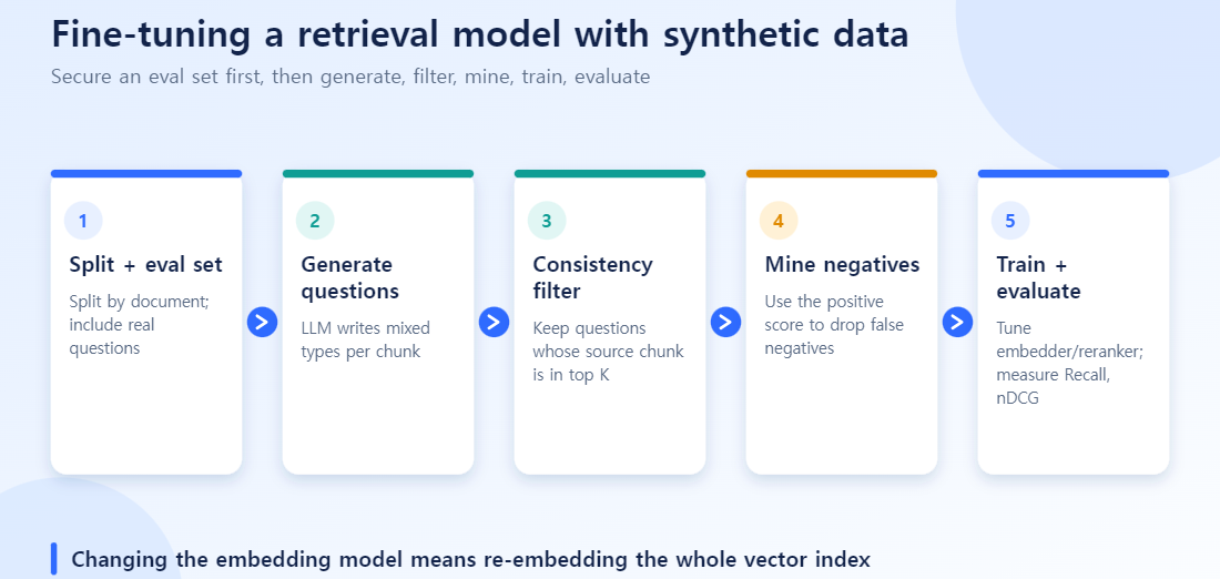
Step 2. Generate questions — mix the types
One question type per chunk narrows the distribution. Specify types (fact lookup, procedure, comparison, short keyword queries) and add a few real internal queries as few-shot examples to match the tone.
PROMPT = """Write {n} questions that can be answered using only the passage below.
- Mix types: fact lookup, procedure, comparison, two-or-three-word keyword queries
- Do not copy sentences from the passage; use wording a user would type
- No general-knowledge questions answerable without the passage
[Real query examples]
{real_queries}
[Passage]
{chunk}
Output a JSON array only."""
Step 3. Consistency filter
def keep(query, chunk_id, retriever, k=5):
    hits = retriever.search(query, top_k=k)
    return chunk_id in {h.id for h in hits}
The pass rate itself is a diagnostic. A very low rate suggests vague questions or bad chunking; a very high rate suggests questions that copy the chunk’s wording and are too easy.
Step 4. Hard-negative mining (positive-aware)
Pull top candidates with the existing embedding, and exclude any whose score is much higher than or close to the positive’s as suspected false negatives.
def mine_negatives(q_vec, pos_score, candidates, margin=0.95, top_n=3):
    # candidates: (chunk_id, score) in descending order, positive excluded
    # keep only those at or below 95% of the positive score -> hard but unlikely to be false negatives
    ok = [(cid, s) for cid, s in candidates if s <= pos_score * margin]
    return [cid for cid, _ in ok[:top_n]]
margin=0.95 is an illustrative starting value, not an answer; tune it to your corpus. Two more safeguards help.
- Exclude chunks from the same document or section: adjacent chunks of the same policy often share the answer.
- Audit a sample: open 50 mined negatives and check by eye that none of them actually answer the question.
Step 5. Fine-tune the embedding model (bi-encoder)
With anchor/positive/negative columns, MNRL also uses the other samples in the batch as negatives.
from datasets import Dataset
from sentence_transformers import SentenceTransformer, SentenceTransformerTrainer, losses

model = SentenceTransformer("BAAI/bge-m3")
train = Dataset.from_dict({"anchor": queries, "positive": pos_chunks, "negative": neg_chunks})
loss = losses.MultipleNegativesRankingLoss(model)
SentenceTransformerTrainer(model=model, train_dataset=train, loss=loss).train()
- The model name and arguments are examples; check the
SentenceTransformerTrainerarguments in the documentation for your sentence-transformers version. - Changing the embedding model means re-embedding the entire existing vector index.
Step 6. Fine-tune the reranker (cross-encoder)
A reranker reads the question and document together, so hard negatives mined with the Step 5 embedding model can feed it directly. If label quality worries you, having an LLM judge “does this document answer the question?” to double-check positives and negatives is an approach used in research.[8] It is usually better to try one of embedding or reranker first and decide the next step from evaluation scores.
Step 7. Evaluate — separate retrieval metrics from answer metrics
| Stage | Metric | What it shows |
|---|---|---|
| First retrieval | Recall@k, MRR | Does the correct chunk make it into the candidates? |
| After reranking | nDCG@k, Precision@k | Is the top ordering right? |
| Final answer | Answer match rate, citation accuracy | Quality as users feel it |
As the ALoFTRAG results show, retrieval metrics can rise while the final answer improves little, so record all three layers separately to see where the gain came from.
How “accuracy went up N%” is actually judged
An accuracy number only means something once you fix what counts as correct, which question set is used, and what it is compared against. The same model can score 60% or 90% depending on those choices.
1. Define “correct” first
| Metric | Definition | Used for |
|---|---|---|
| Recall@k | Share of questions whose correct chunk appears in the top k results | Retrieval stage: “is the answer in the candidates?” |
| MRR | Mean of the reciprocal rank of the first correct chunk (rank 1 = 1, rank 2 = 0.5, …) | How high the correct chunk sits |
| nDCG@k | A 0-to-1 score that accounts for multiple correct chunks and their ranks | Ordering quality after reranking |
| Answer accuracy | Share of generated answers that match the reference answer, graded by humans or an LLM | Quality as users feel it |
A claim like “RAG accuracy is 90%” cannot be compared unless it says which metric it is. Recall@5 and Recall@20 can differ a lot even for the same model.
2. Compare before and after on the same set and conditions
- Freeze the evaluation set. Split it from training data by document, and do not tune settings while looking at it.
- The baseline is the base model before fine-tuning. “Improvement” always means a difference from the baseline.
- Keep chunking, top-k and prompts identical and change only the model, so the effect is isolated.
- Include dozens to hundreds of real user questions where possible. Measuring on synthetic questions alone overstates gains.
3. Distinguish % from percentage points
Suppose Recall@5 goes from 120 of 200 questions (60%) to 138 of 200 (69%):
- Absolute improvement: +9 percentage points (60% to 69%)
- Relative improvement: +15% (9 / 60)
The same result can be described as “9% better” or “15% better”, so you have to check in the source whether a paper’s or vendor’s “+8.3%” is absolute or relative. For ALoFTRAG’s reported average gains of +8.3% citation accuracy and +3.0% answer accuracy, I could not confirm which definition applies in this survey, so check the paper.
4. Check that the gain is not chance
With few evaluation questions the numbers wobble. In the example above, a single 60% figure from 200 questions has a 95% margin of about ±7 percentage points (binomial approximation). A +3-point difference can disappear with a different question set.
- Run both models on the same questions and compare per question (paired comparison). It has less noise than comparing totals.
- Get a confidence interval with bootstrapping (resampling questions repeatedly) or a McNemar test, and do not claim an improvement if the interval includes zero.
- Repeat training with two or three seeds and see whether the result is consistent.
5. For answer accuracy, the grading method is the standard
- Exact or contains-match: objective, but counts differently worded correct answers as wrong.
- LLM grading: fast, but the grader has biases, so first check its agreement with a human-graded sample (for example 50 items).
- Citation accuracy: separately check whether the cited source chunk actually supports the answer. This ties more directly to retrieval improvements.
6. What to report alongside the number
- The metric name and k value (for example Recall@5)
- The number and mix of evaluation questions (synthetic vs. real)
- Baseline and post-tuning values, marked as absolute (points) or relative (%)
- A confidence interval or repeated-run results
- Whether general-query performance held up (a forgetting check)
Without these, “accuracy rose N%” is a number nobody can reproduce.
Check these before fine-tuning
Fine-tuning is the last lever. These come first.
- Have you used logs to tell whether the answer is missing from the candidates (a retrieval problem) or present but not turned into an answer (a generation problem)?
- Have you already applied chunk size and overlap tuning, hybrid search (BM25 + dense) and a reranker?
- Have you tried improvements that need no training data, such as an internal glossary or query expansion?
Common mistakes
- Evaluating only on synthetic questions: train and eval distributions match, so gains are overstated. Mix in real queries.
- Ignoring false negatives: the harder the negative, the more likely it is actually an answer. Do not skip same-document exclusion and sample audits.
- Training on everything without filtering: vague questions become noise. Consistency filtering is a high-value step for its cost.
- Over-relying on LLM-generated negatives: in the text retrieval comparison they did not beat mining. Treat them as a supplement.
- Forgetting the re-embedding cost: replacing the embedding model means rebuilding the whole index.
- Sending confidential documents to an external API for generation: check your data-egress policy before using an external LLM for question generation, and use a local model if the content is sensitive.
Summary
- Synthetic questions plus positive/hard-negative data are a realistic way to adapt a retrieval model to your domain without internal labels.
- Generate, apply a consistency filter, then mine positive-aware negatives: this is the skeleton that recurs across the research.
- Pairs with in-batch negatives are the easy start, triplets add precision on look-alikes, and a mixed setup spends hard negatives only where needed.
- Fine-tuning keeps the model architecture and changes its weights; the loss function and data setup only decide how the weights are adjusted during training.
- Reported gains vary by study, and better retrieval metrics do not automatically mean better final answers, so verify on your own evaluation set.
References
- InPars Toolkit: A Unified and Reproducible Synthetic Data Generation Pipeline for Neural Information Retrieval / InPars-v2
- InPars+: Supercharging Synthetic Data Generation for Information Retrieval Systems
- Dense Text Retrieval based on Pretrained Language Models: A Survey
- NV-Retriever: Improving text embedding models with effective hard-negative mining / RocketQA
- Don’t Retrieve, Generate: Prompting LLMs for Synthetic Training Data in Dense Retrieval
- DocReRank: Single-Page Hard Negative Query Generation for Training Multi-Modal RAG Rerankers
- ALoFTRAG: Automatic Local Fine Tuning for Retrieval Augmented Generation
- Enhancing Transformer-Based Rerankers with Synthetic Data and LLM-Based Supervision
- Sentence Transformers — Natural Language Inference (triplet loss guide)
- In-Batch Negatives — ZeroEntropy (supplementary)
- RocketQA — batch size and false-negative experiments
- Sentence Transformers — Batch Sampler docs
- KaLM-Embedding-V2 — InfoNCE denominator combining in-batch and hard negatives
- Twinkle — InfoNCE Loss (false-negative masking option)